Sports scheduling / Operations research
Rethinking the World Cup schedule
A World Cup schedule determines how far teams travel, how much time they have to recover, and the conditions they play in. It also determines when fans can watch and which cities host the biggest matches.
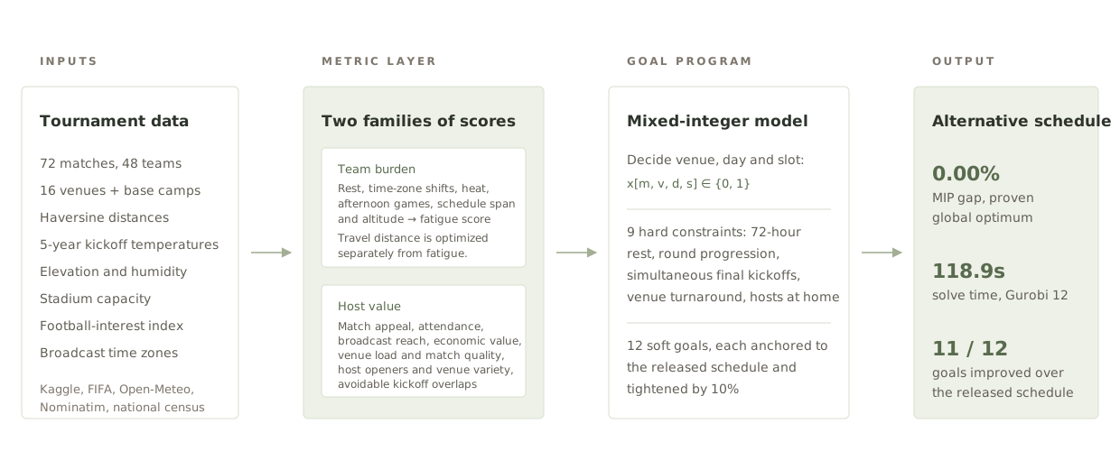
For the CORS OR Challenge, we built a mixed-integer goal program for all 72 group-stage matches. Its 12 goals cover team fairness, travel, broadcast reach, attendance, venue balance, and host-city value, along with host opening matches, venue diversity, and avoidable kickoff overlaps. Rest periods, round order, and venue availability constrain the schedules it can choose.
What the original schedule tells us
Before changing the schedule, we wanted to understand who it worked well for and where it created disadvantages. We examined it from two perspectives: the teams playing the matches and the cities hosting them.
For teams, the burden is not shared equally
Teams in the same group compete for qualification, but can face very different travel distances, time-zone changes, and playing conditions. We compared those differences across five dimensions: travel, time-zone shifts, heat, travel-adjusted rest, and altitude.
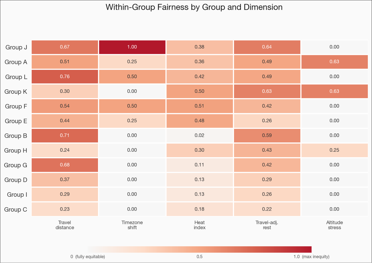
How to read the heatmap
Each cell takes the highest minus the lowest team value within a group, then divides it by the range across all 48 teams. A value of 0 means the teams are equal on that measure. A value of 1 means the group spans the full tournament-wide range. Groups are ordered by the average of their five cell values.
What stood out
Group J spans the full range of time-zone burden, while Group L’s travel spread is 0.76 of the tournament-wide range. Group K has no time-zone disparity but substantial differences in heat, recovery, and altitude. Looking at travel alone would miss those differences.
This is a baseline inequality diagnostic, separate from the optimization model’s weighted fatigue score. Equal burdens can still be high burdens. The heat calculation uses historical kickoff temperatures and an assumed 60% relative humidity.
For hosts, match count is only part of the picture
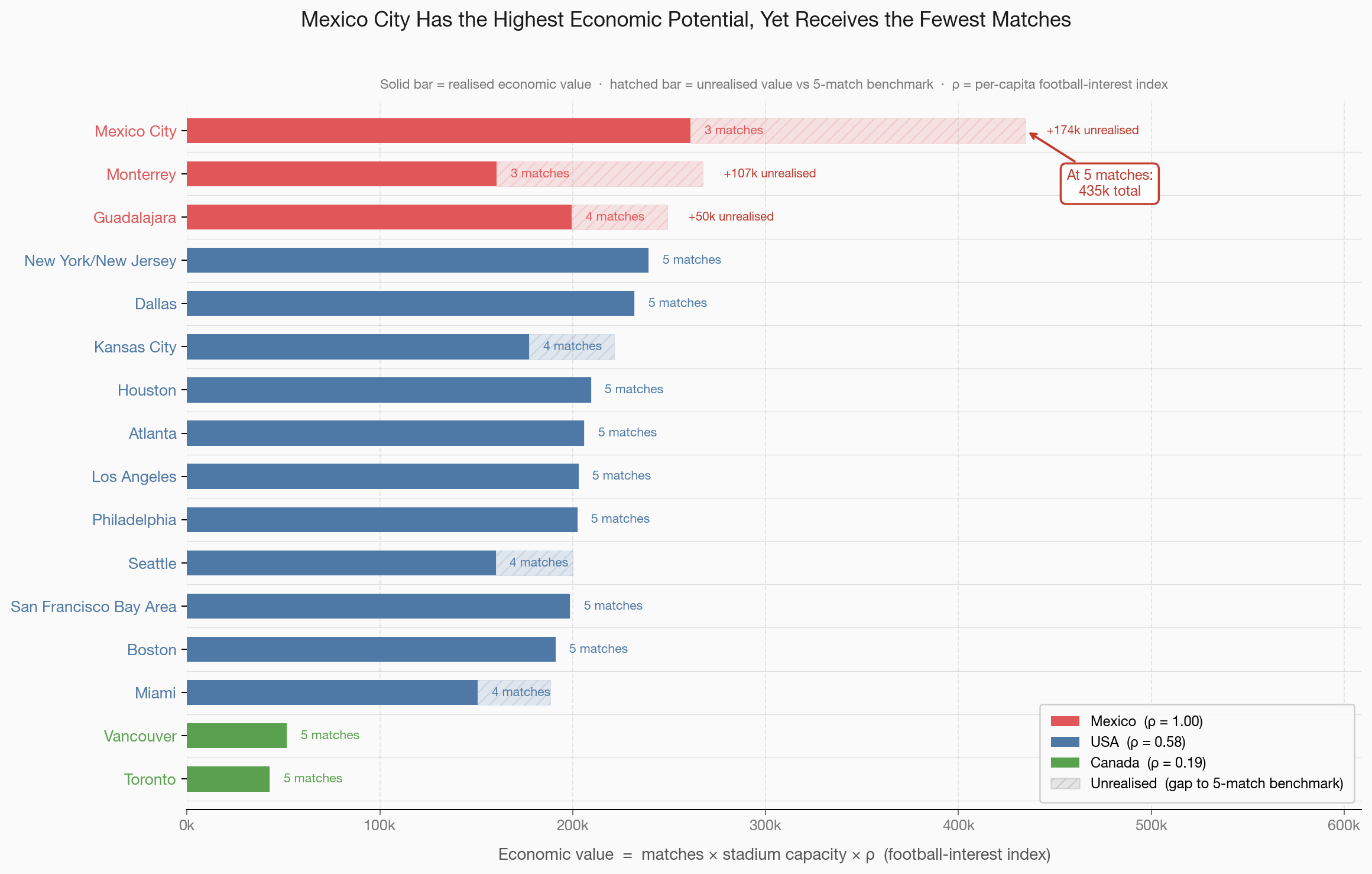
Giving two cities the same number of matches does not necessarily give them the same opportunity. We built a simple host-value score using stadium capacity and a country-level football-interest index, then compared the original allocation with a common five-match benchmark.
Match count × stadium capacity × football-interest index
Where the interest index comes from
We used domestic top-league attendance per person as a proxy for football interest, scaled relative to Mexico. The index is 1.00 for Mexico, 0.58 for the USA, and 0.19 for Canada. It gives the comparison a demand component alongside stadium size.
Why Mexico City stood out
With 87,000 seats, an interest index of 1.00, and three matches in the baseline, Mexico City scores 261,000. Five matches would score 435,000, a gap of 174,000 score units. That prompted us to examine whether different venue assignments could make better use of host capacity.
The five-match benchmark is a diagnostic comparison, not a requirement or a complete feasible schedule. These scores are not revenue estimates, and the chart’s “unrealised” value is a gap in the proxy score rather than lost income.
What could change, and what had to stay fixed
Understanding the scheduling requirements shaped the model. We kept the group draw and match pairings fixed and chose new venues, dates, and kickoff times within the tournament window.
- Fixed base camps
- We treated the supplied base-camp assignments as fixed inputs. Teams return to their assigned camps between matches, so travel is measured as round trips from those locations. The model changes match venues, not where teams are based.
- At least 72 hours between games
- Consecutive matches for each team must have kickoff times at least 72 hours apart. Travel-adjusted rest is assessed separately because the same gap can leave different amounts of recovery time.
- Final group matches start together
- The two matches in each group’s third round share a date and kickoff time, limiting the advantage of knowing the other result. This applies within each group, not to every group at once.
- Time to turn venues around
- A venue hosts at most one match per day, with match dates at least two days apart. This leaves time between fixtures for stadium preparation.
- Round order and local kickoff windows
- Round progression is preserved, and kickoff choices are restricted by venue time zone. Our configuration also caps the daily schedule at six matches.
- Host nations play at home
- Canada, Mexico, and the USA keep their group-stage matches in their own countries. Opening-day placement and the spread of host matches across domestic venues are also represented in the model’s goals.
Choosing among feasible schedules
We brought together travel, historical weather, altitude, stadium capacity, and audience-interest data to score each schedule. We then set targets for 12 goals using the released schedule and fairness thresholds. Mixed-integer goal programming minimizes weighted shortfalls from those targets while enforcing the scheduling constraints.
- Decision variables
- 215,929
- Constraints
- 7,875
- Reported solve time
- 118.9 s
- Reported MIP gap
- 0.00%
Reported Gurobi 12.0 run on Trillium. Global optimality applies to the specified objective, constraints, and input assumptions.
Compare the baseline and optimized schedules
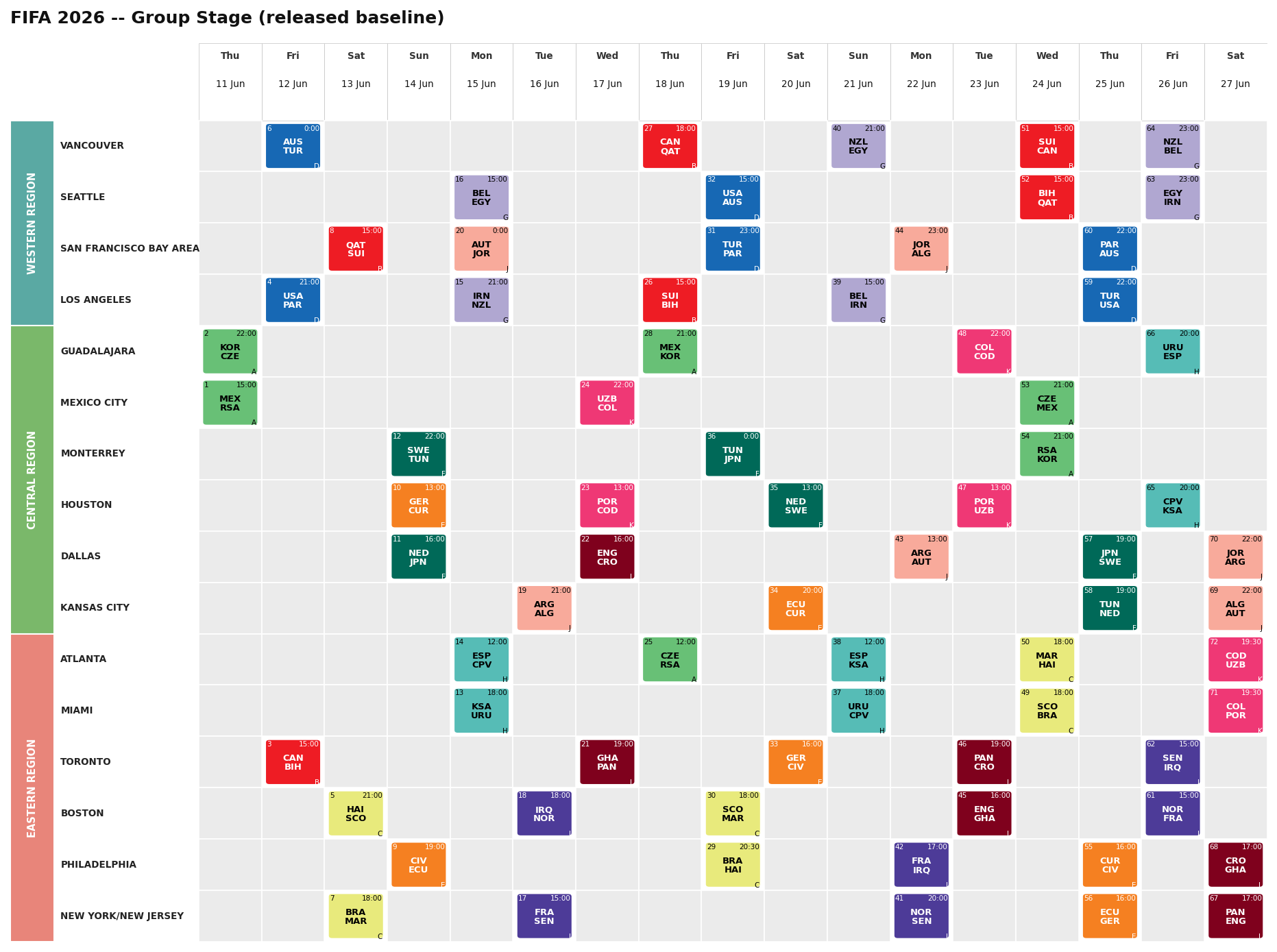
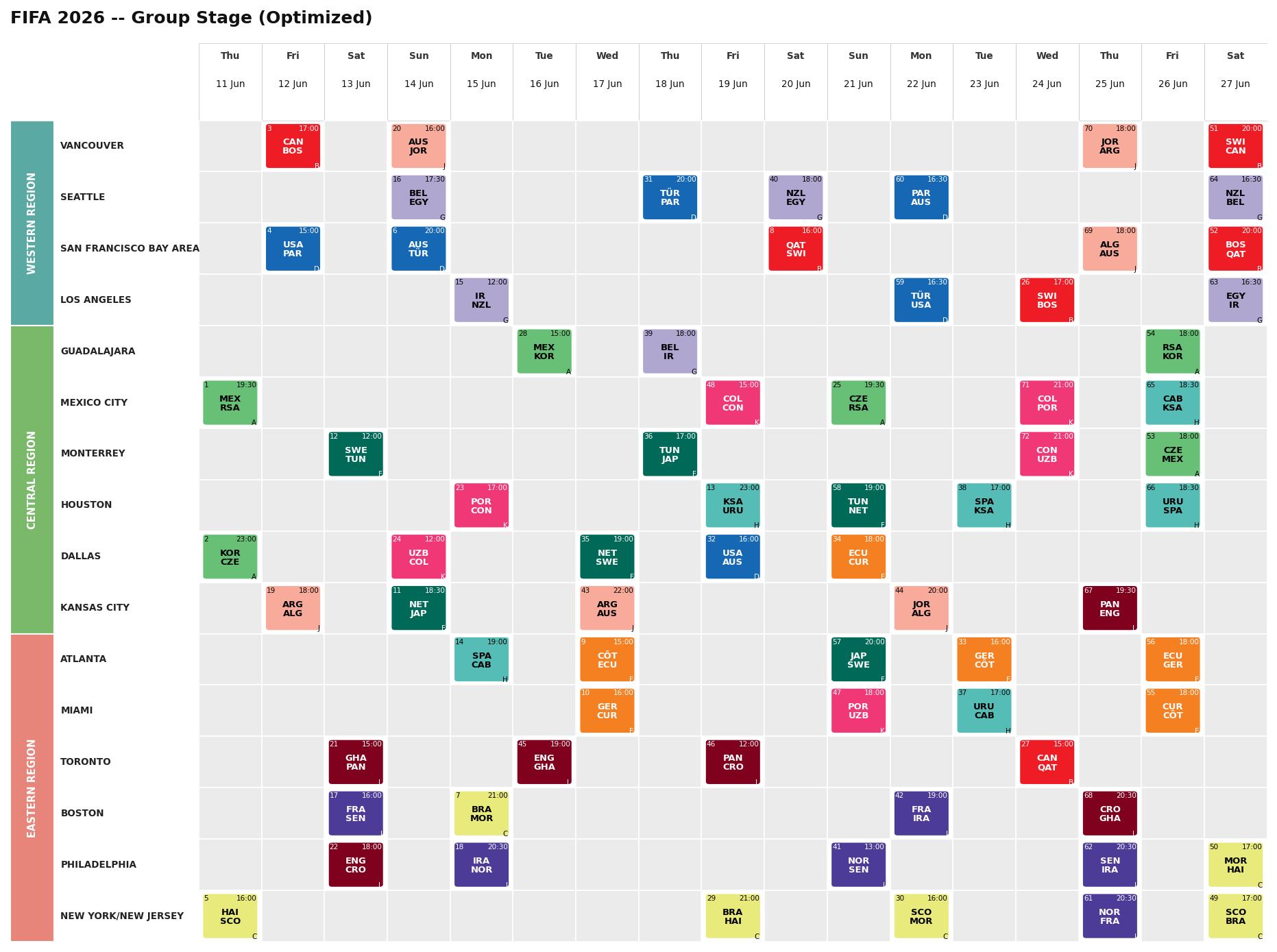
What improved
Our schedule improved 11 of the 12 goals we measured against the released schedule. The remaining goal, avoiding unnecessary match overlaps, was already satisfied and stayed that way.
- Within-group fatigue spread
- −26.2%
- Total base-camp travel
- −10.8%
- Broadcast reach score
- +15.4%
A smaller gap between the most and least burdened teams.
243,380 km → 217,001 km across the tournament.
More suitable kickoff times for fans watching from home.
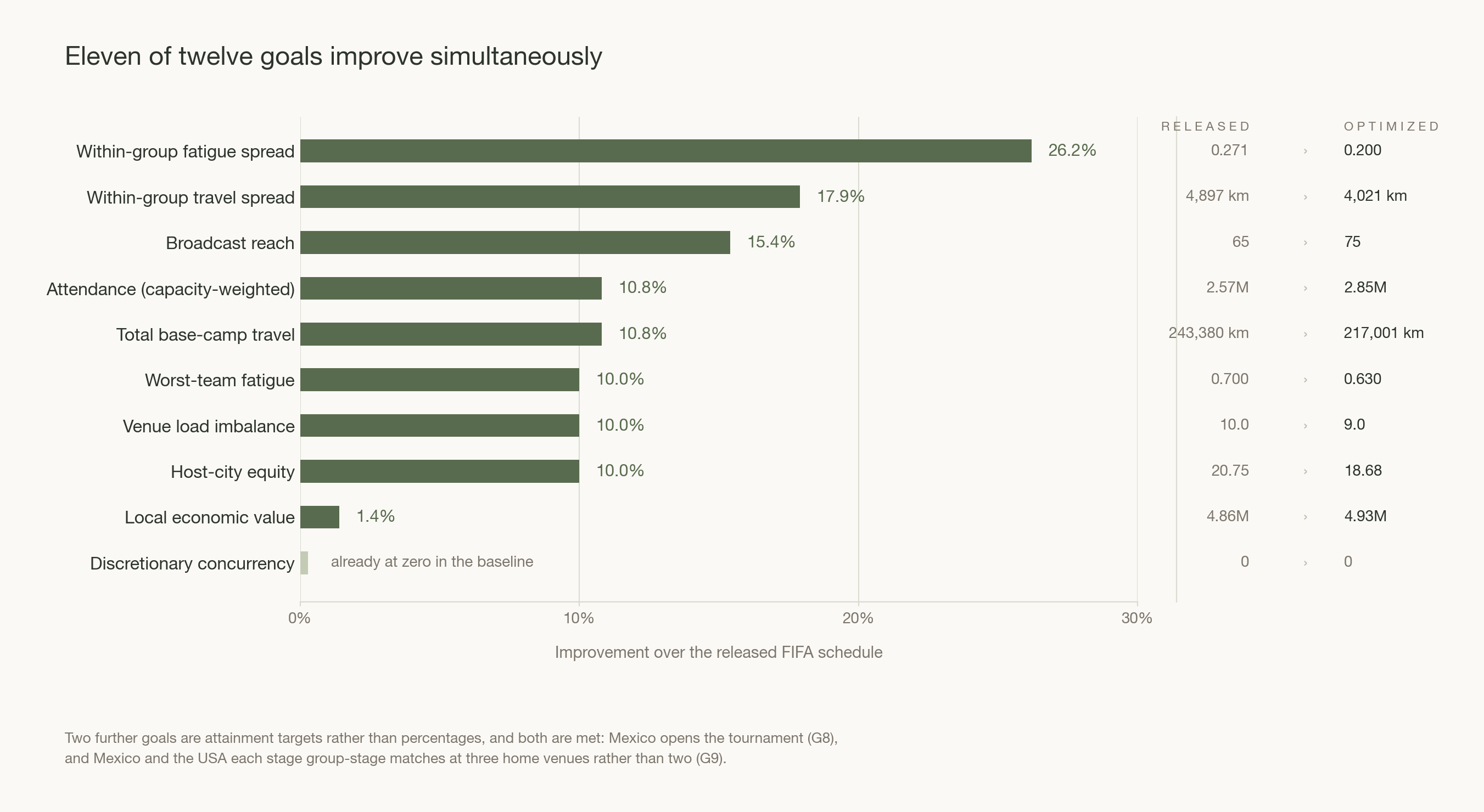
These comparisons use our model’s estimates of fatigue, attendance, broadcast reach, and economic value. They do not measure actual tournament outcomes.
What we learned
I started this project barely knowing how the World Cup group stage worked. I finally have something to contribute to a sports conversation, though hopefully they’re interested in logistics rather than who’s going to win.
Make better use of the venues
Our analysis suggested that Mexican venues could take on a greater role. Changing venue assignments and kickoff times improved the model’s commercial scores while also reducing differences in team fatigue.
Account for travel when measuring rest
Three days off after a long flight gives a team less recovery time than three days in the same city. We gave travel-adjusted rest the largest weight in our fatigue score so the model accounted for that difference.